The Normal Curve
One of the most fundamental concepts in statistics is the normal distribution. It’s often referred to as the bell curve in more informal conversations. Conversely, you may hear it called ‘Gaussian’ in more academic settings. These are all the same concept.
Today’s article will make us Amateurs in the Normal Distribution. Specifically we’re going to learn:
- What is a normal distribution?
- What is standard deviation?
- How to use a normal distribution and standard deviation together to estimate how likely something is to happen
- Applying all this to a real world scenario
Let’s dive in!
The Normal Curve in Theory
The concept behind the normal curve is this:
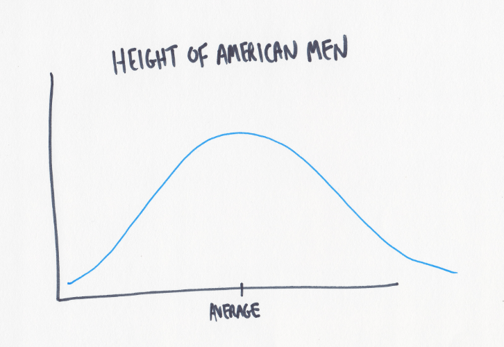
- When you measure something lots of times, like different people’s height, you’ll get a variety of results. Some people are taller and some are shorter, but from these measurements you can calculate an average.
- Some values will be higher than average, some will be lower.
- The higher and lower you go from the average the fewer values you’ll get. There are people who are 7feet tall, but not a lot.
If you collect enough data, the result of these three statements means you get a picture of your data that looks roughly like this.
Standard Deviation – The Map of Your Distribution
An important number related to a normal distribution is what’s called standard deviation. Since we are Amateurs, we won’t dive into the math today. Let’s just say standard deviation is calculated by comparing each of your results to the average of your results. Some of your data points will be closer to the average than others.
Essentially, standard deviation is a measure of how spread out your data is. Some normal curves are tall and skinny, some are short and wide and the standard deviation will be smaller in the first case and bigger in the second.
How Likely Is A Result
What is standard deviation for? We can use it to tell us how likely we are to get a particular result.
Suppose you want to predict how likely you are to find someone of a certain height. Standard deviation will tell you how likely (or unlikely) a single result is to occur. Let’s see how.
Look back at the graph above, specifically the space under the normal distribution and above the horizontal x-axis. This is referred to as the ‘area under the curve’ and, by definition, it’s 100%. Which just means all possible heights can be place as a dot somewhere under that curve.
Let’s add some vertical lines now at one standard deviation above and below the mean. If the average American male is 5’9″ and and standard deviation is 3″ then we have lines and 5’6″ and 6’0″, these are in red. We’ll repeat for two standard deviations, which are 5’3″ and 6’3″ which are in purple.
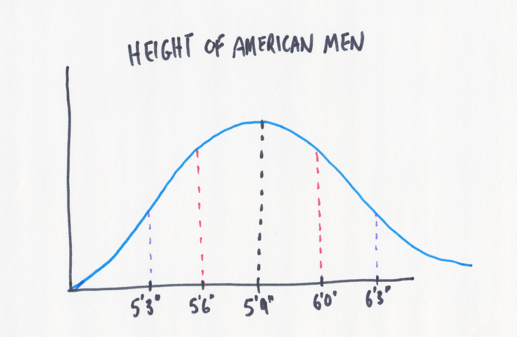
Back to our question, how likely is a certain height? One of the useful results of calculating standard deviation is that a consistent set of rules follows: 68.2% of all your results will be between -1 and 1 standard deviation. About 95.5% of results will be between -2 and 2 standard deviations. This is true of every normal curve.
Practically speaking, this means that if you start picking random American males and measure their height then 68% of the time they will be between 5’6″ and 6’0″.
Or, if you find someone who is exactly 6’3″ you can confidently say he is taller than 98% of all other American men. Why 98% and not 96%? This because the 96% number is the range from 5’3″ to 6’3″. If you want to state the odds of being 6’3″ or more you want to include the people who are under 5’3″ too, so you add in that extra 2% on the left side of the graph; 96%+2%=98%!
The Normal Curve In Practice (How to Use This at Work)
Running a Test
Using the ideas above we can apply them to real scenarios to understand if a result we see is a real impact or not. Imagine you work in your company’s marketing department and the company has just run a test on the website to get customers to spend more money. Pretty common stuff.
A selected group of visitors, randomly picked, were given two different web experiences. Maybe it’s a new color scheme, maybe it’s an easier checkout process, maybe it’s something else. The key is that one group of customers were randomly treated differently than the other.
Now, you have to figure out if that change mattered! Let’s apply what you just learned.
Checking the results
First, you calculate the average spend and standard deviation of the shoppers who did not get the test. Let’s imagine the average is $100 and the standard deviation is $15.
Next, you calculate the average spend of the customers who did receive the test and let’s assume it’s more. It might be $101, or it might be $131 or anything else. (It’s possible that this average will also be exactly $100, but even a little natural variation will give you a different average number since this is a different group of customers.)
Do the Results Matter
Would your test have been successful if the average was $101? What if it was $131? What if it’s just coincidence that the random people you picked to be tested happened to spend more money? How can you know? The standard deviation can tell you.
Let’s add one standard deviation of our control average, which gives us $115. From that we can infer that without the test 84% of shoppers spend $115 or less. Said differently, if our test group has an average spend of $115 there’s a 16% chance that our random group actually ended up picking more of our better customers. There’s a 16% chance it’s coincidence.
Now, if our test group has an average spend of $131 we are two standard deviations away and just like our 6’3″ tall man, we’d get that result by coincidence only 2% of the time. That certainly feels better than 16%! This percentage can be calculated for any average that the test group shows.
Naturally, you’re asking now what percentage is enough to safely say the results are real. Unfortunately, there’s not a single answer for that and it depends on what you’re testing. The levels of confidence required in new drug testing are different than they are for changing the free shipping threshold on a website. You’ll often see 95% put out as a magic number, but in reality even that is just an arbitray choice. We talk on this site about Domain Expertise as one of the 4 Pillars of Data Science and choosing appropriate value is a great example of why.
Conclusion
What’s described above in this testing scenario is very common and you’ll hear it referred to as A/B testing, Hypothesis Testing or t-testing. You’ve learned how data is often naturally spread out. You’ve seen how the amount of that spread can be measured. And finally, once you understand that you’ve seen how you can use that information to test changes in the real world.
This concept, along with my article about Regression Lines, is a core concept that much of Data Science’s statistics are built against. If you understand these two ideas you’re becoming quite an Amateur!
