The Basics of SQL (And Why Amateurs Need to Know It)
Data science is full of different ways to solve the same problems. This is true from the approaches and methods you choose to the languages you code those methods into.
When you’re new to the field it’s natural to try to figure out which language is the best to learn and go learn that one. But there’s not a clear answer to this, meaningful work can be done in Python, R, Matlab, SAS, etc. And if you asked them I suspect most data scientists will tell you the language they use is the one you should also use (and they’ll have a lot of good reasons why that’s the case).
But there’s another language out there that’s sometimes overlooked – SQL. It’s older than R and Python and it’s not a true data science language by itself but if you understand how to write SQL, even just basics, you’ll find a lot of situations where it makes data management significantly easier and faster.
Today’s article is going to teach you the basics of how to read and write SQL. It’s easier than it probably looks right now and by the end of this article you’ll be able to select data from a table in a database; combine it with other tables and create summaries of those tables.
Wait, We’re Coding? I Can’t Even Pronounce SQL!
SQL is an acronym for “Structured Query Language”, which just means a set of rules (structure) that define how to you ask (query) the data something. And let’s get a simple question out of the way – how do you say ‘SQL’. There’s two ways you’ll hear it and they are interchangable: 1) Say each letter S-Q-L just like “TNT” or “OK”. 2) Or say ‘sequel’, just like in the movies. Personally I say ‘sequel’ so you should too!
This article is going to spend more time in code than usual. I typically focus on concepts, intentionally avoiding any code so that Amateurs can think about what’s happening rather than how it’s happening. But SQL is so foundational that it’s important for you to understand both the what and the how.
Tables, Databases and SQL
Before you can write any SQL you need your data stored in tables.
To keep this simple we’re going to make an important assumption – that your data is tabular, meaning that it’s stored in rows and columns. In future articles I’ll spend some time on databases, which are just collections of lots of tables, and why you’d have multiple tables instead of just one huge table. For today, just assume you find your data in separated tables.
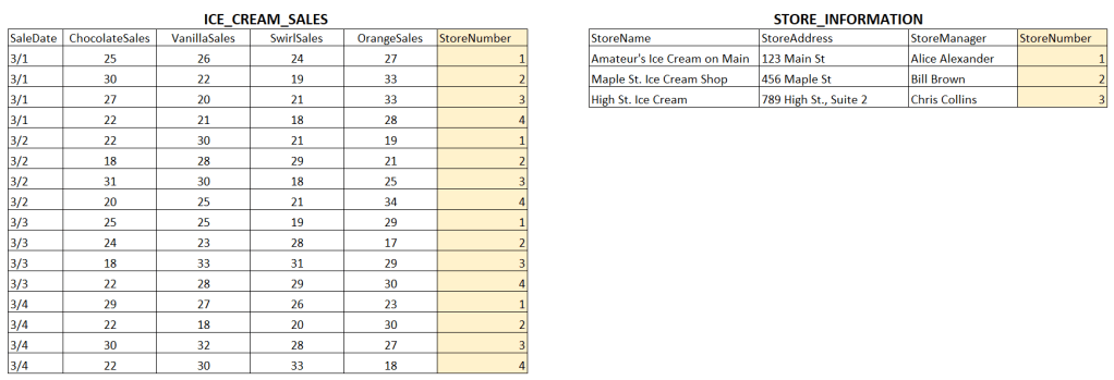
We’re going to start with two tables and we’re going to go back to the Amateur Ice Cream Shop to see its data. Our first table shows sales of ice cream flavors at 4 stores, on 4 different days. The second table just has store information. A couple of columns are yellow, we’ll come back to that.
A Simple Query in Three Steps
1) SELECTing The Data
Every SQL statement has a SELECT section at the top. This is where you list off the columns you want to get back. If you need to see only the date and store of chocolate sales you’d write this:
SELECT SaleDate, StoreNumber, ChocolateSales
2) Data Comes FROM a Table
After your SELECT step you have to tell the database which table you want it to go to for the columns. This is the FROM statement and, added to the SELECT statement above, you get this:
SELECT SaleDate, StoreNumber, ChocolateSales
FROM ICE_CREAM_SALES
And that’s it! This query will work on our database and give you a result that is 3 columns wide and 16 rows long.
3) WHERE You Can Filter
The query above gives you all the rows in the table for those three columns. That’s manageable since we only have 16 rows total. In real life you may not need every row or the table may be too big to do that. The WHERE clause is how you reduce the results to only the rows you need. Let’s say you need to know the chocolate sales for only store number ‘1’:
SELECT SaleDate, StoreNumber, ChocolateSales
FROM ICE_CREAM_SALES
WHERE StoreNumber = '1'
This query will give you all four rows of your data that is related to store number 1. Your WHERE clause doesn’t have to be an ‘=’ value, you can also use write where clauses for greater than, less than, not equal or ‘IN’, a concept that lets you create a list of values you want to use.
Joining More Than One Table
Let’s add a second table to our example. We now have our same table as before and another table that has information about each store. If you are trying to look at sales for each store, like above, getting a list of store numbers might not useful. Instead, printing the store name in your results will make it more readable. Using the JOIN statement is how you do that.
There are different flavors of joins, let’s start with INNER JOIN. These means you will select a column from your first table and match it to the same column in your second table. Remember those columns highlighted in yellow, these are our join keys and we use the “ON” command to tell SQL to use them. This example uses StoreNumber for our matching column.
SELECT SaleDate, a.StoreNumber, ChocolateSales, StoreName
FROM ICE_CREAM_SALES a
INNER JOIN STORE_INFORMATION b
  ON a.StoreNumber = b.StoreNumber
Three things happened here:
- On line 3 I added our second table
- On line 4 I told the database how to match the two tables above by using the ‘ON’ command
- There’s an ‘a’ and ‘b’ after each table name. These are aliases and in the rest of the query anytime I refer to ‘a.’ or ‘b.’ the database knows I mean the respective table (such as in the ON command).
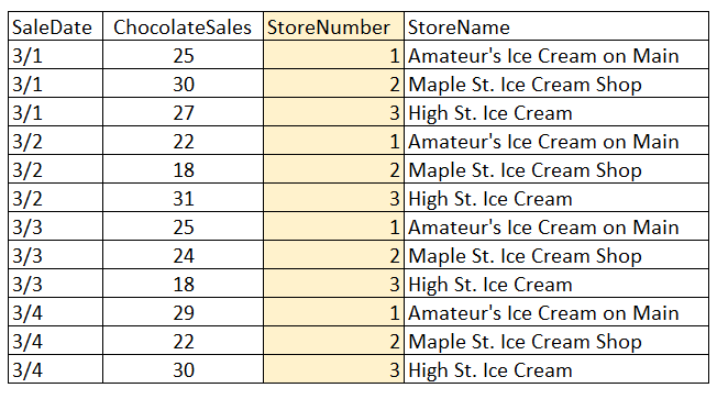
The results are below. Take a look and see if you can follow how everything was put together.
INNER vs OUTER Joins
Do you notice anything that hasn’t worked quite the way we want above? Where is store number 4? An important piece of information about INNER JOINS – it will only give you a result there is a match in both tables. Since store number 4 doesn’t exist in the STORE_INFORMATION table, you won’t get it in your results.
Is that a problem? It depends. If you need to show sales for every store it would be a problem. To solve this we can switch the INNER JOIN to be an OUTER JOIN. This is an easy as it sounds.
SELECT SaleDate, a.StoreNumber, ChocolateSales, StoreName
FROM ICE_CREAM_SALES a
LEFT OUTER JOIN STORE_INFORMATION b
  ON a.StoreNumber = b.StoreNumber
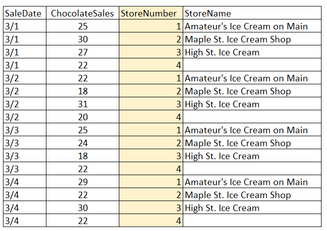
You’ll see I added the words “LEFT OUTER” in place of the word “INNER”. This tells the SQL that you want to take the first table – the ‘left’ table if you put this all on a single line – and that you want to keep everything in that table. Then you want to join it to the ‘right’ table. Since it’s an OUTER join, when there is not a StoreNumber to match on, you still keep your data from the ‘left’ table and no value is put in place where the ‘right’ table would be. It will look like this
Aggregating Your Results
Our results from both the INNER and OUTER joins show the data at a daily level, there are entries for March 1, March 2, etc. There will be many times where you want to aggregate those low level data into something higher. Imagine a question where you need to get the sales of Store Number 1 for last year? You could write a query to give you 365 rows and then you can add those up, but SQL has a faster way.
Built into SQL are many “OLAP” functions. OLAP is an acronym for ‘Online Analytical Processing’ but that’s a mouthful. A simpler explaination is that these are keywords that let you take your results and add them up or find an average or several other common math functions. Let’s look at an example first, trying to sum the Chocolate sales numbers for all four days in our data.
SELECT a.StoreNumber, SUM(ChocolateSales), StoreName
FROM ICE_CREAM_SALES a
LEFT OUTER JOIN STORE_INFORMATION b
  ON a.StoreNumber = b.StoreNumber
GROUP BY a.StoreNumber, StoreName
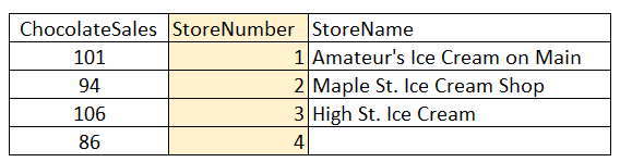
There are only a few changes here. First, I removed SaleDate because we don’t want to see each day anymore. Second, I wrapped the ChocolateSales field with “SUM”. Lastly I added a GROUP BY line at the very end. This tells SQL to combine the common values for StoreNumber and StoreName when doing the SUM on ChocolateSales. The results will be what you see below. (If you’ve ever made a pivot table in Excel, this is essentially what you did!)
There are many of these OLAP function, the most common functions you’ll come across are:
- SUM – adds up the values of the column
- AVG – finds an average of the values in the column
- MIN – get the lowest value in the column
- MAX – get the largest value in the column
- COUNT – counts the number of values in a column
Wrapping It All Up
Today was a longer article about a foundational topic. Once you become comfortable with basic SQL and the table layout that it uses you will begin to think about data in a different way. You learned that SQL requires your data to be in a table layout. You then saw how simple a query can be to see that data, just a few lines. The real power comes from combining multiple tables together with join commands. And finally, once you get your results you know how to perform some basic OLAP functions on it to refine what you get. Master this topic and you’ll not only be an Amateur but well on your way to more!
